studio-lab

Reading a recommender notebook in the open

Applied analysis · 2025

Published
Separator
Author
rhizae
Separator
Last updated

A published Jupyter notebook comparing three recommendation approaches, rendered as readable prose rather than a download.

Tags

  • notebooks
  • recommender-systems
  • reproducibility

A notebook is the honest artifact of an analysis and a poor way to publish one. It carries the code, the data shapes and the intermediate results that make a conclusion checkable, and it usually reaches a reader as a file to download, a rendered image, or a link to a service that may not be there next year.

This page takes the opposite approach. The notebook below is the real thing, pinned to a specific commit, and it is readable before any JavaScript runs.

What is actually on this page

The notebook’s prose, code and text output are all in the HTML this page ships. That matters for three separate reasons, and only one of them is about speed:

  • It can be read without JavaScript, on a slow connection, and by a screen reader that never waits for a renderer to appear. The chart output carries a written description for the same reason Charts that survive without color argues for, since a plot no one can read is not evidence.
  • The site’s own search indexes it, so a phrase from inside the notebook finds this page.
  • It cannot silently change. The file’s checksum is recorded in the repository, and the build refuses to run against anything else.

Once the interactive renderer loads, it replaces that rendition rather than sitting beside it, so nothing here is announced or indexed twice.

Music recommendation reference notebook. Pinned to a specific commit, so this page cannot change underneath its own conclusions.A Jupyter notebook that loads a play-count dataset, explores how often users interact with each title, and compares a popularity baseline against user-user and item-item collaborative filtering.

Music Recommendation System

Problem Definition

The context: Why is this problem important to solve?<br> Music streaming platforms have rapid expanding libraries which produces a major challenge for users. There is not enough time nor energy for the users to find and consume content that is relevant to their taste. To encourage user engagement the best solution is to provide and present content close to the user's taste. Positively engaged users will most likely spend more time on a platform therefore giving the streaming service more chances to increase streams of revenue.

Using the Unified Theory of Acceptance and Use of Technology (UTAUT) researchers have extended the UTAUT model through collected data that categorized contributing factors to user's behavioral intentions. Factors that can be influenced by the product itself are performance expectancy, effort expectancy, hedonic motivation, involvement and interest, and personalization. 1 <br>

The objectives: What is the intended goal?<br> There is a two part objective to this case study. 1) Engage users and personalize their experience and 2) also increase the ease and enjoyment in finding new music. With the context of the UTAUT extended model, achieving this two part objective will increase user engagement and retention but also user recommendations to their peers.<br>

The key questions: What are the key questions that need to be answered?<br> How many different user profiles are there based on similar song selection? What other relationships and patterns occur in the data? What could be the restraints of the solutions we can produce because of the given data? <br>

The problem formulation: What are we trying to solve using data science? The solution we will be driving towards is formulating accurate predictions for new songs based off of a user's song selection history. Data science can solve this problem by building an appropriate recommendation system. Gathering data in this scenario is fairly easy for the streaming platform and it can be gathered in such a way that it strengthens the model. <br>

1* "Music streaming services: understanding the drivers of customer purchase and intention to recommend" Mariana Lopes Barata, Pedro Simões Coelho Aug 2021

Data Dictionary

The core data is the Taste Profile Subset released by the Echo Nest as part of the Million Song Dataset. There are two files in this dataset. The first file contains the details about the song id, titles, release, artist name, and the year of release. The second file contains the user id, song id, and the play count of users.

song_data

song_id - A unique id given to every song

title - Title of the song

Release - Name of the released album

Artist_name - Name of the artist

year - Year of release

count_data

user _id - A unique id given to the user

song_id - A unique id given to the song

play_count - Number of times the song was played

Data Source

http://millionsongdataset.com/

Importing Libraries and the Dataset

# Mounting the drive
from google.colab import drive
drive.mount('/content/drive')
Mounted at /content/drive
# Used to ignore the warning given as output of the code
import warnings
warnings.filterwarnings('ignore')

# Basic libraries of python for numeric and dataframe computations
import numpy as np
import pandas as pd

# Basic library for data visualization
import matplotlib.pyplot as plt

# Slightly advanced library for data visualization
import seaborn as sns

# To compute the cosine similarity between two vectors
from sklearn.metrics.pairwise import cosine_similarity

# A dictionary output that does not raise a key error
from collections import defaultdict

# A performance metrics in sklearn
from sklearn.metrics import mean_squared_error

Load the dataset

# Importing the datasets
count_df = pd.read_csv('/content/drive/MyDrive/count_data.csv')
song_df = pd.read_csv('/content/drive/MyDrive/song_data.csv')
count_df_copy = count_df.copy(deep = True)
song_df_copy = song_df.copy(deep = True)

Understanding the data by viewing a few observations

# See top 10 records of count_df data
count_df_copy.head(n=10)
   Unnamed: 0                                   user_id             song_id  \
0           0  b80344d063b5ccb3212f76538f3d9e43d87dca9e  SOAKIMP12A8C130995   
1           1  b80344d063b5ccb3212f76538f3d9e43d87dca9e  SOBBMDR12A8C13253B   
2           2  b80344d063b5ccb3212f76538f3d9e43d87dca9e  SOBXHDL12A81C204C0   
3           3  b80344d063b5ccb3212f76538f3d9e43d87dca9e  SOBYHAJ12A6701BF1D   
4           4  b80344d063b5ccb3212f76538f3d9e43d87dca9e  SODACBL12A8C13C273   
5           5  b80344d063b5ccb3212f76538f3d9e43d87dca9e  SODDNQT12A6D4F5F7E   
6           6  b80344d063b5ccb3212f76538f3d9e43d87dca9e  SODXRTY12AB0180F3B   
7           7  b80344d063b5ccb3212f76538f3d9e43d87dca9e  SOFGUAY12AB017B0A8   
8           8  b80344d063b5ccb3212f76538f3d9e43d87dca9e  SOFRQTD12A81C233C0   
9           9  b80344d063b5ccb3212f76538f3d9e43d87dca9e  SOHQWYZ12A6D4FA701   

   play_count  
0           1  
1           2  
2           1  
3           1  
4           1  
5           5  
6           1  
7           1  
8           1  
9           1  
# See top 10 records of song_df data
song_df_copy.head(n=10)
              song_id                                              title  \
0  SOQMMHC12AB0180CB8                                       Silent Night   
1  SOVFVAK12A8C1350D9                                        Tanssi vaan   
2  SOGTUKN12AB017F4F1                                  No One Could Ever   
3  SOBNYVR12A8C13558C                                      Si Vos Querés   
4  SOHSBXH12A8C13B0DF                                   Tangle Of Aspens   
5  SOZVAPQ12A8C13B63C  Symphony No. 1 G minor "Sinfonie Serieuse"/All...   
6  SOQVRHI12A6D4FB2D7                                   We Have Got Love   
7  SOEYRFT12AB018936C                                  2 Da Beat Ch'yall   
8  SOPMIYT12A6D4F851E                                            Goodbye   
9  SOJCFMH12A8C13B0C2                         Mama_ mama can't you see ?   

                                release  \
0                 Monster Ballads X-Mas   
1                           Karkuteillä   
2                                Butter   
3                               De Culo   
4  Rene Ablaze Presents Winter Sessions   
5      Berwald: Symphonies Nos. 1/2/3/4   
6             Strictly The Best Vol. 34   
7                               Da Bomb   
8                             Danny Boy   
9  March to cadence with the US marines   

                                      artist_name  year  
0                                Faster Pussy cat  2003  
1                                Karkkiautomaatti  1995  
2                                  Hudson Mohawke  2006  
3                                     Yerba Brava  2003  
4                                      Der Mystic     0  
5                                David Montgomery     0  
6                              Sasha / Turbulence     0  
7                                      Kris Kross  1993  
8                                    Joseph Locke     0  
9  The Sun Harbor's Chorus-Documentary Recordings     0  

Let us check the data types and and missing values of each column

# See the info of the count_df data
print("Missing values: ",count_df_copy.isnull().values.any())
count_df_copy.info(verbose=True, show_counts=True)
Missing values:  False
<class 'pandas.core.frame.DataFrame'>
RangeIndex: 2000000 entries, 0 to 1999999
Data columns (total 4 columns):
 #   Column      Non-Null Count    Dtype 
---  ------      --------------    ----- 
 0   Unnamed: 0  2000000 non-null  int64 
 1   user_id     2000000 non-null  object
 2   song_id     2000000 non-null  object
 3   play_count  2000000 non-null  int64 
dtypes: int64(2), object(2)
memory usage: 61.0+ MB
# See the info of the song_df data
print("Missing values: ", song_df_copy.isnull().values.any())
song_df_copy.info()
Missing values:  True
<class 'pandas.core.frame.DataFrame'>
RangeIndex: 1000000 entries, 0 to 999999
Data columns (total 5 columns):
 #   Column       Non-Null Count    Dtype 
---  ------       --------------    ----- 
 0   song_id      1000000 non-null  object
 1   title        999985 non-null   object
 2   release      999995 non-null   object
 3   artist_name  1000000 non-null  object
 4   year         1000000 non-null  int64 
dtypes: int64(1), object(4)
memory usage: 38.1+ MB

Observations and Insights:

Count Data:

  • The shape of the data is 2000000 rows and 4 columns
  • There are no missing values
  • The columns are split between object type and int64

------ Song Data:

  • The shape of the data is 1000000 rows and 5 columns
  • There are 15 rows missing titles data
  • There are 5 rows missing releases data
  • The columns are all object type except year which is int64
# Left merge the count_df and song_df data on "song_id". Drop duplicates from song_df data simultaneously
df = pd.merge(count_df, song_df, on = 'song_id', how = 'left').drop_duplicates(subset = ['user_id','song_id'])

# Drop the column 'Unnamed: 0'
df = df.drop(['Unnamed: 0'], axis = 1)

print('Number of Duplicates:', df.duplicated(subset = ['user_id','song_id']).sum())
print('Shape of Dataframe:', df.shape)
df.head(10)
Number of Duplicates: 0
Shape of Dataframe: (2000000, 7)
                                     user_id             song_id  play_count  \
0   b80344d063b5ccb3212f76538f3d9e43d87dca9e  SOAKIMP12A8C130995           1   
1   b80344d063b5ccb3212f76538f3d9e43d87dca9e  SOBBMDR12A8C13253B           2   
2   b80344d063b5ccb3212f76538f3d9e43d87dca9e  SOBXHDL12A81C204C0           1   
4   b80344d063b5ccb3212f76538f3d9e43d87dca9e  SOBYHAJ12A6701BF1D           1   
5   b80344d063b5ccb3212f76538f3d9e43d87dca9e  SODACBL12A8C13C273           1   
6   b80344d063b5ccb3212f76538f3d9e43d87dca9e  SODDNQT12A6D4F5F7E           5   
7   b80344d063b5ccb3212f76538f3d9e43d87dca9e  SODXRTY12AB0180F3B           1   
8   b80344d063b5ccb3212f76538f3d9e43d87dca9e  SOFGUAY12AB017B0A8           1   
9   b80344d063b5ccb3212f76538f3d9e43d87dca9e  SOFRQTD12A81C233C0           1   
10  b80344d063b5ccb3212f76538f3d9e43d87dca9e  SOHQWYZ12A6D4FA701           1   

                            title                                release  \
0                        The Cove                     Thicker Than Water   
1                 Entre Dos Aguas                    Flamenco Para Niños   
2                        Stronger                             Graduation   
4                  Constellations                      In Between Dreams   
5                    Learn To Fly          There Is Nothing Left To Lose   
6    Apuesta Por El Rock 'N' Roll                  Antología Audiovisual   
7                   Paper Gangsta                       The Fame Monster   
8                  Stacked Actors          There Is Nothing Left To Lose   
9                   Sehr kosmisch                     Musik von Harmonia   
10  Heaven's gonna burn your eyes  Hôtel Costes 7 by Stéphane Pompougnac   

                                    artist_name  year  
0                                  Jack Johnson     0  
1                                 Paco De Lucia  1976  
2                                    Kanye West  2007  
4                                  Jack Johnson  2005  
5                                  Foo Fighters  1999  
6                           Héroes del Silencio  2007  
7                                     Lady GaGa  2008  
8                                  Foo Fighters  1999  
9                                      Harmonia     0  
10  Thievery Corporation feat. Emiliana Torrini  2002  
from sklearn.preprocessing import LabelEncoder

# Apply label encoding for "user_id" and "song_id"
le = LabelEncoder()
df['user_id'] = le.fit_transform(df['user_id'])
df['song_id'] = le.fit_transform(df['song_id'])
df.head()
   user_id  song_id  play_count            title  \
0    54961      153           1         The Cove   
1    54961      413           2  Entre Dos Aguas   
2    54961      736           1         Stronger   
4    54961      750           1   Constellations   
5    54961     1188           1     Learn To Fly   

                         release    artist_name  year  
0             Thicker Than Water   Jack Johnson     0  
1            Flamenco Para Niños  Paco De Lucia  1976  
2                     Graduation     Kanye West  2007  
4              In Between Dreams   Jack Johnson  2005  
5  There Is Nothing Left To Lose   Foo Fighters  1999  
# Get the column containing the users
users = df.user_id

# Create a dictionary from users to their number of songs
ratings_count = dict()

for user in users:
    # If we already have the user, just add 1 to their rating count
    if user in ratings_count:
        ratings_count[user] += 1

    # Otherwise, set their rating count to 1
    else:
        ratings_count[user] = 1
# We want our users to have listened at least 90 songs
RATINGS_CUTOFF = 90

# Create a list of users who need to be removed
remove_users = []

for user, num_ratings in ratings_count.items():

    if num_ratings < RATINGS_CUTOFF:
        remove_users.append(user)

df = df.loc[ ~ df.user_id.isin(remove_users)]
# Get the column containing the songs
songs = df.song_id

# Create a dictionary from songs to their number of users
ratings_count = dict()

for song in songs:
    # If we already have the song, just add 1 to their rating count
    if song in ratings_count:
        ratings_count[song] += 1

    # Otherwise, set their rating count to 1
    else:
        ratings_count[song] = 1
# We want our song to be listened by atleast 120 users to be considred
RATINGS_CUTOFF = 120

remove_songs = []

for song, num_ratings in ratings_count.items():
    if num_ratings < RATINGS_CUTOFF:
        remove_songs.append(song)

df_final= df.loc[ ~ df.song_id.isin(remove_songs)]
# Drop records with play_count more than(>) 5
df_final = df_final[df_final["play_count"] <= 5]
# Check the shape of the data
rows, columns = df_final.shape
print("No of rows: ", rows)
print("No of columns: ", columns)
df_final.info()
No of rows:  117876
No of columns:  7
<class 'pandas.core.frame.DataFrame'>
Int64Index: 117876 entries, 209 to 2086699
Data columns (total 7 columns):
 #   Column       Non-Null Count   Dtype 
---  ------       --------------   ----- 
 0   user_id      117876 non-null  int64 
 1   song_id      117876 non-null  int64 
 2   play_count   117876 non-null  int64 
 3   title        117876 non-null  object
 4   release      117876 non-null  object
 5   artist_name  117876 non-null  object
 6   year         117876 non-null  int64 
dtypes: int64(4), object(3)
memory usage: 7.2+ MB

Exploratory Data Analysis

Data Description

  • Background of the data and what is it about?
  • The data is the Taste Profile Subset released by the Echo Nest as part of the Million Song Dataset. It shows the relationship of song consumption by users.
  • Information about the variables included in the data
  • There are two data sets, Count Data and Song Data. The count data shows the user's interaction with one song. The song data gives a description of that song. There is no description of the user other than the user ID.

------ Observations & Insights

  • What are some key patterns observed in the data during EDA?
  • There is a left skew in songs played vs songs released
  • How do the key patterns affect/relate to the problem?
  • This might signal a bias because streamed music started in late 1990 and early 2000
  • What are the data treatments or pre-processing steps required, if any?
  • Combined the data sets, removed the users and items that had incredibly low interaction, dropped duplicates we did not want to consider, and removed any large player counts that would weigh too heavily in creating a rating.

Let's check the total number of unique users, songs, artists in the data

Total number of unique user id

# Display total number of unique user_id
print('Number of unique USERS in the final data = ', df_final['user_id'].nunique())
Number of unique USERS in the final data =  3155

Total number of unique song id

# Display total number of unique song_id
print('Number of unique SONGS in the final data = ', df_final['song_id'].nunique())
Number of unique SONGS in the final data =  563

Total number of unique artists

# Display total number of unique artists
print('Number of unique ARTISTS in the final data = ', df_final['artist_name'].nunique())
Number of unique ARTISTS in the final data =  232
print('The number of observations in the final data = ', len(df_final))
The number of observations in the final data =  117876

Observations and Insights:

  • There are 400730 observations
  • There are 2992 unique users
  • There are 8111 unique songs
  • There are 2998 unique artists

----

  • There are 24,268,112 possible interactions
  • On average users interacted with any song 133 times
  • On average song interacted with any user 49 times
  • Users are interacting with multiple songs
  • Songs are being interacted with multiple times
  • The numeric gap between the possible interactions and actual observations creates a possibility of building a recommendation system

Let's find out about the most interacted songs and interacted users

Most interacted songs

print('Most interacted songs =  \n', df_final['song_id'].value_counts())
Most interacted songs =  
 8582    751
352     748
2220    713
1118    662
4152    652
       ... 
9048    103
6450    102
990     101
4831     97
8324     96
Name: song_id, Length: 563, dtype: int64

Most interacted users

print('Most interacted users = \n', df_final['user_id'].value_counts())
Most interacted users = 
 61472    243
15733    227
37049    202
9570     184
23337    177
        ... 
19776      1
45476      1
17961      1
14439      1
10412      1
Name: user_id, Length: 3155, dtype: int64

Observations and Insights: The most songs that have been interacted by a user is 621 which is far from the actual number of songs in the present data. We can build a recommendation system to recommend songs to users. The most users that have interacted with a song is 751, therefore we can also recommend popular items to users as well.

Songs played in a year
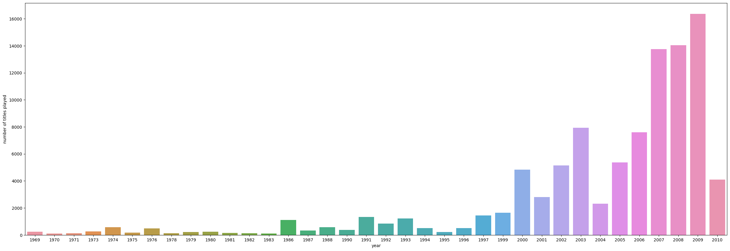
count_songs = df_final.groupby('year').count()['title']

count = pd.DataFrame(count_songs)

count.drop(count.index[0], inplace = True)

count.tail()
      title
year       
2006   7592
2007  13750
2008  14031
2009  16351
2010   4087
# Create the plot

# Set the figure size
plt.figure(figsize = (30, 10))

sns.barplot(x = count.index,
            y = 'title',
            data = count,
            estimator = np.median)

# Set the y label of the plot
plt.ylabel('number of titles played')

# Show the plot
plt.show()
A bar chart of the median number of plays per title, showing a long tail in which most titles are played only a handful of times while a small number account for most listening.

Observations and Insights: There is a significant left skew of the data. There is a possibility since streaming became more relevant towards the 2000s that songs that were released during that time had a higher probability to be streamed by the demographic targeted by the platform. There may be a bias where the popularity of a song is affected by the age of release and the emergence of streamed music.

Proposed approach

Potential techniques: What different techniques should be explored?<br>

  • Rank Based Recommendation System
  • Collaborative Filtering Based Recommendation System
  • Model Based Collaborative Filtering Recommendation System

Given the data at hand where we only have data about the user - song interaction that it would be appropriate to experiment with these types of techniques.

Overall solution design: What is the potential solution design?<br> Each potential technique will be created and then optimized with optimal hyperparameters using Surprise and Scikit Learn. We then will compare and choose based on our measures of success.

Measures of success: What are the key measures of success to compare different potential techniques?<br>

  • Precision
  • Recall
  • F1-Score

Precision and Recall are both important in this situation, so focusing on optimizing for the F1-Score will be the best option.

Popularity-Based Recommendation Systems

Let's take the count and sum of play counts of the songs and build the popularity recommendation systems based on the sum of play counts.

# Calculating average play_count
average_count = df_final.groupby('song_id').mean()['play_count']        # Hint: Use groupby function on the song_id column

# Calculating the frequency a song is played
play_freq = df_final.groupby('song_id').count()['play_count']         # Hint: Use groupby function on the song_id column
# Making a dataframe with the average_count and play_freq
final_play = pd.DataFrame({'avg_count': average_count, 'play_freq': play_freq})

# Let us see the first five records of the final_play dataset
final_play.head()
         avg_count  play_freq
song_id                      
21        1.622642        265
22        1.492424        132
52        1.729216        421
62        1.728070        114
93        1.452174        115

Now, let's create a function to find the top n songs for a recommendation based on the average play count of song. We can also add a threshold for a minimum number of playcounts for a song to be considered for recommendation.

# Build the function to find top n songs

# It gives top n songs among those being watched for more than min_interactions
def top_n_songs(data, n, min_interaction = 100):

    # Finding songs with interactions greater than the minimum number of interactions
    recommendations = data[data['play_freq'] > min_interaction]

    # Sorting values with respect to the average rating
    recommendations = recommendations.sort_values(by = 'avg_count', ascending = False)

    return recommendations.index[:n]
# Recommend top 10 songs using the function defined above
list(top_n_songs(final_play, 10, 50))
[7224, 8324, 6450, 9942, 5531, 5653, 8483, 2220, 657, 614]
# Recommend top 10 songs using the function defined above
list(top_n_songs(final_play, 10, 100))
[7224, 6450, 9942, 5531, 5653, 8483, 2220, 657, 614, 352]
# Recommend top 10 songs using the function defined above
list(top_n_songs(final_play, 10, 200))
[5531, 2220, 614, 352, 1664, 6246, 4448, 1334, 8019, 7496]

User User Similarity-Based Collaborative Filtering

To build the user-user-similarity-based and subsequent models we will use the "surprise" library.

# Install the surprise package using pip. Uncomment and run the below code to do the same
!pip install surprise
Collecting surprise
  Downloading surprise-0.1-py2.py3-none-any.whl (1.8 kB)
Collecting scikit-surprise (from surprise)
  Downloading scikit-surprise-1.1.3.tar.gz (771 kB)
     ━━━━━━━━━━━━━━━━━━━━━━━━━━━━━━━━━━━━━━ 772.0/772.0 kB 13.6 MB/s eta 0:00:00
[?25h  Preparing metadata (setup.py) ... [?25l[?25hdone
Requirement already satisfied: joblib>=1.0.0 in /usr/local/lib/python3.10/dist-packages (from scikit-surprise->surprise) (1.2.0)
Requirement already satisfied: numpy>=1.17.3 in /usr/local/lib/python3.10/dist-packages (from scikit-surprise->surprise) (1.22.4)
Requirement already satisfied: scipy>=1.3.2 in /usr/local/lib/python3.10/dist-packages (from scikit-surprise->surprise) (1.10.1)
Building wheels for collected packages: scikit-surprise
  Building wheel for scikit-surprise (setup.py) ... [?25l[?25hdone
  Created wheel for scikit-surprise: filename=scikit_surprise-1.1.3-cp310-cp310-linux_x86_64.whl size=3096342 sha256=c467f873288df29f289e29afa5b3b924d2fc25b6a85679f1d91c66bff3234e4a
  Stored in directory: /root/.cache/pip/wheels/a5/ca/a8/4e28def53797fdc4363ca4af740db15a9c2f1595ebc51fb445
Successfully built scikit-surprise
Installing collected packages: scikit-surprise, surprise
Successfully installed scikit-surprise-1.1.3 surprise-0.1
# Import necessary libraries

# To compute the accuracy of models
from surprise import accuracy

# This class is used to parse a file containing play_counts, data should be in structure - user; item; play_count
from surprise.reader import Reader

# Class for loading datasets
from surprise.dataset import Dataset

# For tuning model hyperparameters
from surprise.model_selection import GridSearchCV

# For splitting the data in train and test dataset
from surprise.model_selection import train_test_split

# For implementing similarity-based recommendation system
from surprise.prediction_algorithms.knns import KNNBasic

# For implementing matrix factorization based recommendation system
from surprise.prediction_algorithms.matrix_factorization import SVD

# For implementing KFold cross-validation
from surprise.model_selection import KFold

# For implementing clustering-based recommendation system
from surprise import CoClustering

Some useful functions

Below is the function to calculate precision@k and recall@k, RMSE and F1_Score@k to evaluate the model performance.

# The function to calulate the RMSE, precision@k, recall@k, and F_1 score
def precision_recall_at_k(model, k = 30, threshold = 1.5):
    """Return precision and recall at k metrics for each user"""

    # First map the predictions to each user.
    user_est_true = defaultdict(list)

    # Making predictions on the test data
    predictions=model.test(testset)

    for uid, _, true_r, est, _ in predictions:
        user_est_true[uid].append((est, true_r))

    precisions = dict()
    recalls = dict()
    for uid, user_ratings in user_est_true.items():

        # Sort user ratings by estimated value
        user_ratings.sort(key = lambda x : x[0], reverse = True)

        # Number of relevant items
        n_rel = sum((true_r >= threshold) for (_, true_r) in user_ratings)

        # Number of recommended items in top k
        n_rec_k = sum((est >= threshold) for (est, _) in user_ratings[ : k])

        # Number of relevant and recommended items in top k
        n_rel_and_rec_k = sum(((true_r >= threshold) and (est >= threshold))
                              for (est, true_r) in user_ratings[ : k])

        # Precision@K: Proportion of recommended items that are relevant
        # When n_rec_k is 0, Precision is undefined. We here set Precision to 0 when n_rec_k is 0

        precisions[uid] = n_rel_and_rec_k / n_rec_k if n_rec_k != 0 else 0

        # Recall@K: Proportion of relevant items that are recommended
        # When n_rel is 0, Recall is undefined. We here set Recall to 0 when n_rel is 0

        recalls[uid] = n_rel_and_rec_k / n_rel if n_rel != 0 else 0

    # Mean of all the predicted precisions are calculated
    precision = round((sum(prec for prec in precisions.values()) / len(precisions)), 3)

    # Mean of all the predicted recalls are calculated
    recall = round((sum(rec for rec in recalls.values()) / len(recalls)), 3)

    accuracy.rmse(predictions)

    # Command to print the overall precision
    print('Precision: ', precision)

    # Command to print the overall recall
    print('Recall: ', recall)

    # Formula to compute the F-1 score
    print('F_1 score: ', round((2 * precision * recall) / (precision + recall), 3))
# Instantiating Reader scale with expected rating scale
reader = Reader(rating_scale=(0, 5)) #use rating scale (0, 5)

# Loading the dataset
data = Dataset.load_from_df(df_final[["user_id", "song_id", "play_count"]], reader) # Take only "user_id","song_id", and "play_count"

# Splitting the data into train and test dataset
trainset, testset = train_test_split(data, test_size=0.4, random_state = 42) # Take test_size = 0.4
# Build the default user-user-similarity model
sim_options = {'name': 'cosine',
               'user_based':True}

# KNN algorithm is used to find desired similar items
sim_user_user = KNNBasic(sim_options = sim_options, verbose = False, random_state = 1) # Use random_state = 1

# Train the algorithm on the trainset, and predict play_count for the testset
sim_user_user.fit(trainset)

# Let us compute precision@k, recall@k, and f_1 score with k = 30
precision_recall_at_k(sim_user_user) # Use sim_user_user model
RMSE: 1.0878
Precision:  0.396
Recall:  0.692
F_1 score:  0.504

Observations and Insights:

  • The calculated RMSE checks how far the overall predicted counts are from the actual counts
  • Intuition of Precision: Calculated precision is ~0.40
  • 40% out of all the recommended songs are relevant
  • Intuition of Recall: Calculated recall is ~0.69
  • 69% out of all the relevant movies are recommended
  • F1 score baseline ~0.50
  • 50% of mostly recommended items were relevant and relevant items were recommended.
  • We will try to improve this by using GridSearchCV by tuning different hyperparameters

| | User_User | |-----------------|-----------| | RSME | 1.0878 | | Precision | 0.396 | | Recall | 0.692 | | F1 Score | 0.504 | | Prediction Diff | ~0.2 |

# Predicting play_count for a sample user with a listened song
sim_user_user.predict(6958, 1671, r_ui = 2, verbose = True) # Use user id 6958 and song_id 1671
user: 6958       item: 1671       r_ui = 2.00   est = 1.80   {'actual_k': 40, 'was_impossible': False}
Prediction(uid=6958, iid=1671, r_ui=2, est=1.8009387435128914, details={'actual_k': 40, 'was_impossible': False})
# Predicting play_count for a sample user with a song not-listened by the user
sim_user_user.predict(6958, 3232, verbose = True) # Use user_id 6958 and song_id 3232
user: 6958       item: 3232       r_ui = None   est = 1.64   {'actual_k': 40, 'was_impossible': False}
Prediction(uid=6958, iid=3232, r_ui=None, est=1.6386860897998294, details={'actual_k': 40, 'was_impossible': False})

Observations and Insights:

  • The above output shows that the actual play count for this user-item pair is 2, and the predicted play count is ~1.8 by this user-user similarity based baseline model.
  • The output also contains "actual_k". It is the K value in KNN that is used while training, the default value is 40.

Now, let's try to tune the model and see if we can improve the model performance.

# Setting up parameter grid to tune the hyperparameters
param_grid = {'k': [30, 40, 50], 'min_k': [3, 6, 9],
              'sim_options': {'name': ['msd', 'cosine', 'pearson',"pearson_baseline"],
                              'user_based': [True], "min_support":[2,4]}
              }

# Performing 3-fold cross-validation to tune the hyperparameters
gs = GridSearchCV(KNNBasic, param_grid, measures = ['rmse'], cv = 3, n_jobs = -1)

# Fitting the data
gs.fit(data) # Use entire data for GridSearch

# Best RMSE score
print(gs.best_score['rmse'])
# Combination of parameters that gave the best RMSE score
print(gs.best_params['rmse'])
1.0465563863896452
{'k': 50, 'min_k': 9, 'sim_options': {'name': 'pearson_baseline', 'user_based': True, 'min_support': 2}}
# Train the best model found in above gridsearch
# Using the optimal similarity measure for user-user collaborative filtering
sim_options = {'name': 'pearson_baseline',
               'user_based': True,
               'min_support': 2}

# Creating an instance of KNNBasic with optimal hyperparameter values
sim_user_user_optimized = KNNBasic(sim_options=sim_options, k=30, min_k=9, random_state=1, verbose=False)

# Training the algorithm on the train set
sim_user_user_optimized.fit(trainset)

# Let us compute precision@k, recall@k, and F_1 score with k = 10
precision_recall_at_k(sim_user_user_optimized)
RMSE: 1.0521
Precision:  0.413
Recall:  0.721
F_1 score:  0.525

Observations and Insights:

  • We can see after tuning the hyperparameters:
  • ↑ RMSE increased by ~0.04
  • ↑ Precision intuition increased by ~0.02
  • ↑ Recall intuition increased by ~0.03
  • ↓ F_1 score decreased by by ~0.02
  • We can say overall the performance does not have a noticeable improvement

| | User_User | User_User_Opt | |-----------------|-----------|---------------| | RSME | 1.0878 | 1.0521 | | Precision | 0.396 | 0.413 | | Recall | 0.692 | 0.721 | | F1 Score | 0.504 | 0.525 | | Prediction Diff | ~0.2 | ~0.04 |

# Predict the play count for a user who has listened to the song. Take user_id 6958, song_id 1671 and r_ui = 2
sim_user_user_optimized.predict(6958, 1671, r_ui = 2, verbose=True)
user: 6958       item: 1671       r_ui = 2.00   est = 1.96   {'actual_k': 24, 'was_impossible': False}
Prediction(uid=6958, iid=1671, r_ui=2, est=1.962926073914969, details={'actual_k': 24, 'was_impossible': False})
# Predict the play count for a song that is not listened to by the user (with user_id 6958)
sim_user_user_optimized.predict(6958, 3232, verbose=True)
user: 6958       item: 3232       r_ui = None   est = 1.45   {'actual_k': 10, 'was_impossible': False}
Prediction(uid=6958, iid=3232, r_ui=None, est=1.4516261428486725, details={'actual_k': 10, 'was_impossible': False})

Observations and Insights:

  • The above output shows that the actual play count for this user-item pair is 2, and the predicted play count is ~1.96 by this user-user similarity based optimized model.
  • ~0.04 difference of error
  • Tuning of the hyperparameters decreased the difference of error by ~0.16
# Use inner id 0
sim_user_user_optimized.get_neighbors(0,5)
[42, 1131, 17, 186, 249]

Below we will be implementing a function where the input parameters are:

  • data: A song dataset
  • user_id: A user-id against which we want the recommendations
  • top_n: The number of songs we want to recommend
  • algo: The algorithm we want to use for predicting the play_count
  • The output of the function is a set of top_n items recommended for the given user_id based on the given algorithm
def get_recommendations(data, user_id, top_n, algo):

    # Creating an empty list to store the recommended product ids
    recommendations = []

    # Creating an user item interactions matrix
    user_item_interactions_matrix = data.pivot_table(index = 'user_id', columns = 'song_id', values = 'play_count')

    # Extracting those business ids which the user_id has not visited yet
    non_interacted_products = user_item_interactions_matrix.loc[user_id][user_item_interactions_matrix.loc[user_id].isnull()].index.tolist()

    # Looping through each of the business ids which user_id has not interacted yet
    for item_id in non_interacted_products:

        # Predicting the ratings for those non visited restaurant ids by this user
        est = algo.predict(user_id, item_id).est

        # Appending the predicted ratings
        recommendations.append((item_id, est))

    # Sorting the predicted ratings in descending order
    recommendations.sort(key = lambda x : x[1], reverse = True)

    return recommendations[:top_n] # Returing top n highest predicted rating products for this user
# Make top 5 recommendations for user_id 6958 with a similarity-based recommendation engine
recommendations = get_recommendations(df_final, 6958, 5, sim_user_user_optimized)
# Building the dataframe for above recommendations with columns "song_id" and "predicted_ratings"
pd.DataFrame(recommendations, columns=['song_id', 'predicted_play_count'])
   song_id  predicted_play_count
0     5531              2.553335
1      317              2.518269
2     4954              2.406776
3     8635              2.396606
4     5943              2.390723

Observations and Insights: The top five recommended songs have a predicted play count of >2. This can be interpreted that the songs will be played again therefore enough for user engagement and increasing time spent on the application.

Correcting the play_counts and Ranking the above songs

def ranking_songs(recommendations, final_rating):
  # Sort the songs based on play counts
  ranked_songs = final_rating.loc[[items[0] for items in recommendations]].sort_values('play_freq', ascending = False)[['play_freq']].reset_index()

  # Merge with the recommended songs to get predicted play_count
  ranked_songs = ranked_songs.merge(pd.DataFrame(recommendations, columns = ['song_id', 'predicted_play_count']), on = 'song_id', how = 'inner')

  # Rank the songs based on corrected play_counts
  ranked_songs['corrected_play_count'] = ranked_songs['predicted_play_count'] - 1 / np.sqrt(ranked_songs['play_freq'])

  # Difference
  ranked_songs['play_count_difference'] = ranked_songs['predicted_play_count'] - ranked_songs['corrected_play_count']

  # Sort the songs based on corrected play_counts
  ranked_songs = ranked_songs.sort_values('corrected_play_count', ascending = False)

  return ranked_songs
# Applying the ranking_songs function on the final_play data
print(ranking_songs(recommendations, final_play)['play_count_difference'].mean())
ranking_songs(recommendations, final_play)
0.058483597104098804
   song_id  play_freq  predicted_play_count  corrected_play_count  \
0     5531        618              2.553335              2.513109   
2      317        411              2.518269              2.468943   
1     5943        423              2.390723              2.342101   
3     4954        183              2.406776              2.332854   
4     8635        155              2.396606              2.316284   

   play_count_difference  
0               0.040226  
2               0.049326  
1               0.048622  
3               0.073922  
4               0.080322  

Observations and Insights: After calculating the corrected play count - on average there is a difference of ~0.06 from the predicted play count, which is not an impactable difference. The predicted play count is slightly higher than the corrected play count.

Item Item Similarity-based collaborative filtering recommendation systems

# Apply the item-item similarity collaborative filtering model with random_state = 1 and evaluate the model performance
# Declaring the similarity options
sim_options = {'name': 'cosine',
               'user_based': False}

# KNN algorithm is used to find desired similar items
sim_item_item = KNNBasic(sim_options = sim_options, random_state = 1, verbose = False)

# Train the algorithm on the train set, and predict ratings for the test set
sim_item_item.fit(trainset)

# Let us compute precision@k, recall@k, and f_1 score with k = 10
precision_recall_at_k(sim_item_item)
RMSE: 1.0394
Precision:  0.307
Recall:  0.562
F_1 score:  0.397

Observations and Insights:

  • The calculated RMSE checks how far the overall predicted counts are from the actual counts
  • Intuition of Precision: Calculated precision is ~0.30
  • 30% out of all the recommended songs are relevant
  • Intuition of Recall: Calculated recall is ~0.56
  • 56% out of all the relevant movies are recommended
  • F1 score baseline ~0.40
  • 40% of mostly recommended items were relevant and relevant items were recommended.
  • We will try to improve this by using GridSearchCV by tuning different hyperparameters

| | User_User | User_User_Opt | Item_Item | |-----------------|-----------|---------------|-----------| | RSME | 1.0878 | 1.0521 | 1.0394 | | Precision | 0.396 | 0.413 | 0.307 | | Recall | 0.692 | 0.721 | 0.562 | | F1 Score | 0.504 | 0.525 | 0.397 | | Prediction Diff | ~0.2 | ~0.04 | ~0.64 |

# Predicting play count for a sample user_id 6958 and song (with song_id 1671) heard by the user
sim_item_item.predict(6958, 1671, r_ui=2, verbose=True)
user: 6958       item: 1671       r_ui = 2.00   est = 1.36   {'actual_k': 20, 'was_impossible': False}
Prediction(uid=6958, iid=1671, r_ui=2, est=1.3614157231762556, details={'actual_k': 20, 'was_impossible': False})
# Predict the play count for a user that has not listened to the song (with song_id 1671)
sim_item_item.predict(6958, 3232, verbose=True)
user: 6958       item: 3232       r_ui = None   est = 1.38   {'actual_k': 20, 'was_impossible': False}
Prediction(uid=6958, iid=3232, r_ui=None, est=1.377602711737415, details={'actual_k': 20, 'was_impossible': False})

Observations and Insights:

  • The above output shows that the actual play count for this user-item pair is 2, and the predicted play count is ~1.36 by this item-item similarity based baseline model.
  • Item-item similarity model prediction seems to perform not as well with a difference of ~0.64 to the actual play count. (Difference of ~0.44 compared to the user-user similarity model)
# Apply grid search for enhancing model performance

# Setting up parameter grid to tune the hyperparameters
param_grid = {'k': [10, 20, 30], 'min_k': [3, 6, 9],
              'sim_options': {'name': ["cosine", 'pearson', "pearson_baseline"],
                              'user_based': [False], "min_support": [2, 4]}
              }

# Performing 3-fold cross-validation to tune the hyperparameters
gs = GridSearchCV(KNNBasic, param_grid, measures = ['rmse'], cv = 3, n_jobs = -1)

# Fitting the data
gs.fit(data)

# Find the best RMSE score
print(gs.best_score['rmse'])
# Extract the combination of parameters that gave the best RMSE score
print(gs.best_params['rmse'])
1.023373689573307
{'k': 30, 'min_k': 6, 'sim_options': {'name': 'pearson_baseline', 'user_based': False, 'min_support': 2}}
# Apply the best modle found in the grid search
# Using the optimal similarity measure for user-user collaborative filtering
sim_options = {'name': 'pearson_baseline',
               'user_based': False,
               'min_support': 2}

# Creating an instance of KNNBasic with optimal hyperparameter values
sim_item_item_optimized = KNNBasic(sim_options=sim_options, k=30, min_k=6, random_state=1, verbose=False)

# Training the algorithm on the train set
sim_item_item_optimized.fit(trainset)

# Let us compute precision@k, recall@k, and F_1 score with k = 10
precision_recall_at_k(sim_item_item_optimized)
RMSE: 1.0328
Precision:  0.408
Recall:  0.665
F_1 score:  0.506

Observations and Insights:

  • We can see after tuning the hyperparameters:
  • ↓ RMSE decreased by ~0.01
  • ↑ Precision intuition increased by ~0.1
  • ↑ Recall intuition increased by ~0.1
  • ↑ F_1 score increased by by ~0.1
  • We can say overall the performance slightly improved and is comparable to user-user optimized model, however has lower performance ratings.

| | User_User | User_User_Opt | Item_Item | Item_Item_Opt | |-----------------|-----------|---------------|-----------|---------------| | RSME | 1.0878 | 1.0521 | 1.0394 | 1.0328 | | Precision | 0.396 | 0.413 | 0.307 | 0.408 | | Recall | 0.692 | 0.721 | 0.562 | 0.665 | | F1 Score | 0.504 | 0.525 | 0.397 | 0.506 | | Prediction Diff | ~0.2 | ~0.04 | ~0.64 | ~0.04 |

# Predict the play_count by a user(user_id 6958) for the song (song_id 1671)
sim_item_item_optimized.predict(6958, 1671, r_ui=2, verbose=True)
user: 6958       item: 1671       r_ui = 2.00   est = 1.96   {'actual_k': 10, 'was_impossible': False}
Prediction(uid=6958, iid=1671, r_ui=2, est=1.9634957386781853, details={'actual_k': 10, 'was_impossible': False})
# Predicting play count for a sample user_id 6958 with song_id 3232 which is not heard by the user
sim_item_item_optimized.predict(6958, 3232, verbose=True)
user: 6958       item: 3232       r_ui = None   est = 1.28   {'actual_k': 10, 'was_impossible': False}
Prediction(uid=6958, iid=3232, r_ui=None, est=1.2759946618244609, details={'actual_k': 10, 'was_impossible': False})

Observations and Insights:

  • The above output shows that the actual play count for this user-item pair is 2, and the predicted play count is ~1.96 by this item-item similarity based optimized model.
  • ~0.04 difference of error
  • Tuning of the hyperparameters decreased the difference of error by ~0.6
# Find five most similar items to the item with inner id 0
sim_item_item_optimized.get_neighbors(0, 5)
[124, 523, 173, 205, 65]
# Making top 5 recommendations for user_id 6958 with item_item_similarity-based recommendation engine
recommendations = get_recommendations(df_final, 6958, 5, sim_item_item_optimized)
# Building the dataframe for above recommendations with columns "song_id" and "predicted_play_count"
pd.DataFrame(recommendations, columns=['song_id', 'predicted_play_count'])
   song_id  predicted_play_count
0     2342              2.653903
1     5101              2.386577
2      139              2.313727
3     7519              2.270864
4     8099              2.212702
# Applying the ranking_songs function
print(ranking_songs(recommendations, final_play)['play_count_difference'].mean())
ranking_songs(recommendations, final_play)
0.08234907902107444
   song_id  play_freq  predicted_play_count  corrected_play_count  \
4     2342        111              2.653903              2.558987   
2     5101        130              2.386577              2.298871   
3      139        119              2.313727              2.222057   
1     7519        168              2.270864              2.193712   
0     8099        275              2.212702              2.152399   

   play_count_difference  
4               0.094916  
2               0.087706  
3               0.091670  
1               0.077152  
0               0.060302  

Observations and Insights: After calculating the corrected play count - on average there is a difference of ~0.08 from the predicted play count, which is not an impactable difference. The predicted play count is slightly higher than the corrected play count.

Model Based Collaborative Filtering - Matrix Factorization

Model-based Collaborative Filtering is a personalized recommendation system, the recommendations are based on the past behavior of the user and it is not dependent on any additional information. We use latent features to find recommendations for each user.

# Build baseline model using svd
# Using SVD matrix factorization
svd = SVD(random_state = 1)

# Training the algorithm on the train set
svd.fit(trainset)

# Use the function precision_recall_at_k to compute precision@k, recall@k, F1-Score, and RMSE
precision_recall_at_k(svd)
RMSE: 1.0252
Precision:  0.41
Recall:  0.633
F_1 score:  0.498
# Making prediction for user (with user_id 6958) to song (with song_id 1671), take r_ui = 2
svd.predict("6958", "1671", r_ui = 2, verbose = True)
user: 6958       item: 1671       r_ui = 2.00   est = 1.70   {'was_impossible': False}
Prediction(uid='6958', iid='1671', r_ui=2, est=1.6989607635206787, details={'was_impossible': False})
# Making a prediction for the user who has not listened to the song (song_id 3232)
svd.predict("6958", "3232", verbose = True)
user: 6958       item: 3232       r_ui = None   est = 1.70   {'was_impossible': False}
Prediction(uid='6958', iid='3232', r_ui=None, est=1.6989607635206787, details={'was_impossible': False})
Improving matrix factorization based recommendation system by tuning its hyperparameters
# Set the parameter space to tune
param_grid = {'n_epochs': [10, 20, 30], 'lr_all': [0.001, 0.005, 0.01],
              'reg_all': [0.2, 0.4, 0.6]}

# Performe 3-fold grid-search cross-validation
gs = GridSearchCV(SVD, param_grid, measures = ['rmse'], cv = 3, n_jobs = -1)

# Fitting data
gs.fit(data)
# Best RMSE score
print(gs.best_score['rmse'])
# Combination of parameters that gave the best RMSE score
print(gs.best_params['rmse'])
1.0120665373570124
{'n_epochs': 30, 'lr_all': 0.01, 'reg_all': 0.2}
# Building the optimized SVD model using optimal hyperparameters
svd_optimized = SVD(n_epochs=30, lr_all=0.01, reg_all=0.2, random_state=1)

# Train the algorithm on the train set
svd_optimized = svd_optimized.fit(trainset)

# Use the function precision_recall_at_k to compute precision@k, recall@k, F1-Score, and RMSE
precision_recall_at_k(svd_optimized)
RMSE: 1.0141
Precision:  0.415
Recall:  0.635
F_1 score:  0.502

Observations and Insights: Matrix Factorization:

  • The calculated RMSE checks how far the overall predicted counts are from the actual counts
  • Intuition of Precision: Calculated precision is ~0.41
  • 41% out of all the recommended songs are relevant
  • Intuition of Recall: Calculated recall is ~0.63
  • 63% out of all the relevant movies are recommended
  • F1 score baseline ~0.50
  • 50% of mostly recommended items were relevant and relevant items were recommended.

----- Matrix Factorization Optimized:

  • We can see after tuning the hyperparameters:
  • ↑ RMSE decreased by ~0.01
  • [-] Precision intuition did not increase or decrease significantly
  • [-] Recall intuition did not increase or decrease significantly
  • ↓ F_1 score increased by by ~0.01
  • We can say overall the performance does not have a noticeable improvement

| | User_User | User_User_Opt | Item_Item | Item_Item_Opt | Matrix_Factor | Matrix_Factor_Opt | |-----------------|-----------|---------------|-----------|---------------|---------------|-------------------| | RSME | 1.0878 | 1.0521 | 1.0394 | 1.0328 | 1.0252 | 1.0141 | | Precision | 0.396 | 0.413 | 0.307 | 0.408 | 0.41 | 0.415 | | Recall | 0.692 | 0.721 | 0.562 | 0.665 | 0.633 | 0.635 | | F1 Score | 0.504 | 0.525 | 0.397 | 0.506 | 0.498 | 0.502 | | Prediction Diff | ~0.2 | ~0.04 | ~0.64 | ~0.04 | ~0.3 | ~0.3 |

# Using svd_algo_optimized model to recommend for userId 6958 and song_id 1671
svd_optimized.predict('6958', '1671', r_ui=2, verbose=True)
user: 6958       item: 1671       r_ui = 2.00   est = 1.70   {'was_impossible': False}
Prediction(uid='6958', iid='1671', r_ui=2, est=1.6989607635206787, details={'was_impossible': False})
# Using svd_algo_optimized model to recommend for userId 6958 and song_id 3232 with unknown baseline rating
svd_optimized.predict('6958', '3232', verbose=True)
user: 6958       item: 3232       r_ui = None   est = 1.70   {'was_impossible': False}
Prediction(uid='6958', iid='3232', r_ui=None, est=1.6989607635206787, details={'was_impossible': False})

Observations and Insights:

  • The above output shows that the actual play count for this user-item pair is 2, and the predicted play count is ~1.70 by this matrix factorization based optimized model.
  • ~0.3 difference of error
  • Tuning of the hyperparameters did not increase or decrease the performance significantly
  • Although the performance metrics seem comparable to better predicting models, the difference in predicted to actual play count is slightly significant
# Getting top 5 recommendations for user_id 6958 using "svd_optimized" algorithm
svd_recommendations = get_recommendations(df_final, 6958, 5, svd_optimized)
# Ranking songs based on above recommendations
print(ranking_songs(svd_recommendations, final_play)['play_count_difference'].mean())
ranking_songs(svd_recommendations, final_play)
0.09512503575518197
   song_id  play_freq  predicted_play_count  corrected_play_count  \
2     7224        107              2.601899              2.505225   
1     5653        108              2.108728              2.012502   
4     8324         96              2.014091              1.912029   
0     9942        150              1.940115              1.858465   
3     6450        102              1.952493              1.853478   

   play_count_difference  
2               0.096674  
1               0.096225  
4               0.102062  
0               0.081650  
3               0.099015  

Observations and Insights: After calculating the corrected play count - on average there is a difference of ~0.09 from the predicted play count, which is not an impactable difference. The predicted play count is slightly lower than the corrected play count.

Cluster Based Recommendation System

In clustering-based recommendation systems, we explore the similarities and differences in people's tastes in songs based on how they rate different songs. We cluster similar users together and recommend songs to a user based on play_counts from other users in the same cluster.

# Make baseline clustering model
clust_baseline = CoClustering(random_state=1)

# Train the algorithm on the train set
clust_baseline.fit(trainset)

# Compute precision@k, recall@k, and F_1 score with k = 10
precision_recall_at_k(clust_baseline)
RMSE: 1.0487
Precision:  0.397
Recall:  0.582
F_1 score:  0.472
# Making prediction for user_id 6958 and song_id 1671
clust_baseline.predict(6958, 1671, r_ui=2, verbose=True)
user: 6958       item: 1671       r_ui = 2.00   est = 1.29   {'was_impossible': False}
Prediction(uid=6958, iid=1671, r_ui=2, est=1.2941824757363074, details={'was_impossible': False})
# Making prediction for user (userid 6958) for a song(song_id 3232) not heard by the user
clust_baseline.predict(6958, 3232, verbose=True)
user: 6958       item: 3232       r_ui = None   est = 1.48   {'was_impossible': False}
Prediction(uid=6958, iid=3232, r_ui=None, est=1.4785259100797417, details={'was_impossible': False})
Improving clustering-based recommendation system by tuning its hyper-parameters
# Set the parameter space to tune
param_grid = {'n_cltr_u': [3, 4, 5 ], 'n_cltr_i': [3, 4, 5 ], 'n_epochs': [20, 30, 40]}

# Performing 3-fold grid search cross-validation
gs = GridSearchCV(CoClustering, param_grid, measures=['rmse'], cv=3, n_jobs=-1)
# Fitting data
gs.fit(data)
# Best RMSE score
print(gs.best_score['rmse'])

# Combination of parameters that gave the best RMSE score
print(gs.best_params['rmse'])
1.045479087353365
{'n_cltr_u': 3, 'n_cltr_i': 3, 'n_epochs': 30}
# Train the tuned Coclustering algorithm
clust_tuned = CoClustering(n_cltr_u=5,n_cltr_i=5, n_epochs=10, random_state=1)

clust_tuned.fit(trainset)

precision_recall_at_k(clust_tuned)
RMSE: 1.0654
Precision:  0.394
Recall:  0.566
F_1 score:  0.465

Observations and Insights: Clustering:

  • The calculated RMSE checks how far the overall predicted counts are from the actual counts
  • Intuition of Precision: Calculated precision is ~0.40
  • 40% out of all the recommended songs are relevant
  • Intuition of Recall: Calculated recall is ~0.6
  • 60% out of all the relevant movies are recommended
  • F1 score baseline ~0.47
  • 47% of mostly recommended items were relevant and relevant items were recommended.

----- Clustering Optimized:

  • We can see after tuning the hyperparameters:
  • ↑ RMSE increased by by ~0.02
  • [-] Precision intuition did not increase or decrease significantly
  • ↓ Recall intuition decreased by ~0.01
  • [-] F_1 score did not increase or decrease significantly
  • We can say overall the performance does not have a noticeable improvement in the performance metric

| | User_User | User_User_Opt | Item_Item | Item_Item_Opt | Matrix_Factor | Matrix_Factor_Opt | Clustering | Clustering_Opt | |-----------------|-----------|---------------|-----------|---------------|---------------|-------------------|------------|----------------| | RSME | 1.0878 | 1.0521 | 1.0394 | 1.0328 | 1.0252 | 1.0141 | 1.0487 | 1.0654 | | Precision | 0.396 | 0.413 | 0.307 | 0.408 | 0.41 | 0.415 | 0.397 | 0.394 | | Recall | 0.692 | 0.721 | 0.562 | 0.665 | 0.633 | 0.635 | 0.582 | 0.566 | | F1 Score | 0.504 | 0.525 | 0.397 | 0.506 | 0.498 | 0.502 | 0.472 | 0.465 | | Prediction Diff | ~0.2 | ~0.04 | ~0.64 | ~0.04 | ~0.3 | ~0.3 | ~0.71 | ~0.09 |

# Using co_clustering_optimized model to recommend for userId 6958 and song_id 1671
clust_tuned.predict(6958, 1671, r_ui=2, verbose=True)
user: 6958       item: 1671       r_ui = 2.00   est = 1.91   {'was_impossible': False}
Prediction(uid=6958, iid=1671, r_ui=2, est=1.9108882530486497, details={'was_impossible': False})
# Use Co_clustering based optimized model to recommend for userId 6958 and song_id 3232 with unknown baseline rating
clust_tuned.predict(6958, 3232, verbose=True)
user: 6958       item: 3232       r_ui = None   est = 1.24   {'was_impossible': False}
Prediction(uid=6958, iid=3232, r_ui=None, est=1.2366916027865822, details={'was_impossible': False})

Observations and Insights:

  • The above output shows that the actual play count for this user-item pair is 2, and the predicted play count is ~1.91 by this matrix factorization based optimized model.
  • ~0.09 difference of error
  • Tuning of the hyperparameters did increase the performance slightly
  • Although the performance metrics seem on the lower bound compared to the other predictive models, the difference in predicted to actual play count is comparable to the other better performing models.
Implementing the recommendation algorithm based on optimized CoClustering model
# Getting top 5 recommendations for user_id 6958 using "Co-clustering based optimized" algorithm
clustering_recommendations = get_recommendations(df_final, 6958, 5, clust_tuned)

Correcting the play_count and Ranking the above songs

# Ranking songs based on the above recommendations
print(ranking_songs(clustering_recommendations, final_play)['play_count_difference'].mean())
ranking_songs(clustering_recommendations, final_play)
0.08827351600728806
   song_id  play_freq  predicted_play_count  corrected_play_count  \
4     7224        107              3.711503              3.614829   
3     5653        108              2.903883              2.807658   
0     6860        169              2.691043              2.614120   
1      657        151              2.606354              2.524975   
2     8483        123              2.582807              2.492640   

   play_count_difference  
4               0.096674  
3               0.096225  
0               0.076923  
1               0.081379  
2               0.090167  

Observations and Insights: After calculating the corrected play count - on average there is a difference of ~0.09 from the predicted play count, which is not an impactable difference. The predicted play count is slightly lower than the corrected play count.

Content Based Recommendation Systems

df_small = df_final
# Concatenate the "title", "release", "artist_name" columns to create a different column named "text"
df_small['text']=df_small['title'].astype(str)+' '+df_small['release']+' '+df_small['artist_name']
df_small.head()
     user_id  song_id  play_count                            title  \
209     6958      447           1               Daisy And Prudence   
211     6958      512           1  The Ballad of Michael Valentine   
212     6958      549           1        I Stand Corrected (Album)   
213     6958      703           1            They Might Follow You   
214     6958      719           1                       Monkey Man   

                  release      artist_name  year  \
209          Distillation     Erin McKeown  2000   
211               Sawdust      The Killers  2004   
212       Vampire Weekend  Vampire Weekend  2007   
213           Tiny Vipers      Tiny Vipers  2007   
214  You Know I'm No Good    Amy Winehouse  2007   

                                                  text  
209       Daisy And Prudence Distillation Erin McKeown  
211  The Ballad of Michael Valentine Sawdust The Ki...  
212  I Stand Corrected (Album) Vampire Weekend Vamp...  
213      They Might Follow You Tiny Vipers Tiny Vipers  
214      Monkey Man You Know I'm No Good Amy Winehouse  
# Select the columns 'user_id', 'song_id', 'play_count', 'title', 'text' from df_small data
col_names = ['user_id', 'song_id', 'play_count', 'title', 'text']
df_small = df_small[col_names]
# Drop the duplicates from the title column
df_small = df_small.drop_duplicates(subset = ['title'], keep = 'first')
# Set the title column as the index
df_small = df_small.set_index('title')
# See the first 5 records of the df_small dataset
df_small.head()
                                 user_id  song_id  play_count  \
title                                                           
Daisy And Prudence                  6958      447           1   
The Ballad of Michael Valentine     6958      512           1   
I Stand Corrected (Album)           6958      549           1   
They Might Follow You               6958      703           1   
Monkey Man                          6958      719           1   

                                                                              text  
title                                                                               
Daisy And Prudence                    Daisy And Prudence Distillation Erin McKeown  
The Ballad of Michael Valentine  The Ballad of Michael Valentine Sawdust The Ki...  
I Stand Corrected (Album)        I Stand Corrected (Album) Vampire Weekend Vamp...  
They Might Follow You                They Might Follow You Tiny Vipers Tiny Vipers  
Monkey Man                           Monkey Man You Know I'm No Good Amy Winehouse  
# Create the series of indices from the data
indices =pd.Series(df_small.index)

indices[ : 5]
0                 Daisy And Prudence
1    The Ballad of Michael Valentine
2          I Stand Corrected (Album)
3              They Might Follow You
4                         Monkey Man
Name: title, dtype: object
# Importing necessary packages to work with text data
import nltk

# Download punkt library
nltk.download("punkt")

# Download stopwords library
nltk.download("stopwords")

# Download wordnet
nltk.download("wordnet")

# Download omw-1.4
nltk.download('omw-1.4')

# Import regular expression
import re

# Import word_tokenizer
from nltk import word_tokenize

# Import WordNetLemmatizer
from nltk.stem import WordNetLemmatizer

# Import stopwords
from nltk.corpus import stopwords

# Import CountVectorizer and TfidfVectorizer
from sklearn.feature_extraction.text import CountVectorizer, TfidfVectorizer
[nltk_data] Downloading package punkt to /root/nltk_data...
[nltk_data]   Unzipping tokenizers/punkt.zip.
[nltk_data] Downloading package stopwords to /root/nltk_data...
[nltk_data]   Unzipping corpora/stopwords.zip.
[nltk_data] Downloading package wordnet to /root/nltk_data...
[nltk_data] Downloading package omw-1.4 to /root/nltk_data...

We will create a function to pre-process the text data:

# Function to tokenize the text
def tokenize(text):

    text = re.sub(r"[^a-zA-Z]"," ", text.lower())

    tokens = word_tokenize(text)

    words = [word for word in tokens if word not in stopwords.words("english")]  # Use stopwords of english

    text_lems = [WordNetLemmatizer().lemmatize(lem).strip() for lem in words]

    return text_lems
# Create tfidf vectorizer
tfidf = TfidfVectorizer(tokenizer=tokenize)
# Fit_transfrom the above vectorizer on the text column and then convert the output into an array
df_tfidf = tfidf.fit_transform(df_small['text'].values).toarray()
# Compute the cosine similarity for the tfidf above output
similar_songs = cosine_similarity(df_tfidf, df_tfidf)
pd.DataFrame(similar_songs)
     0    1    2    3    4    5    6         7         8    9    ...  551  \
0    1.0  0.0  0.0  0.0  0.0  0.0  0.0  0.281738  0.000000  0.0  ...  0.0   
1    0.0  1.0  0.0  0.0  0.0  0.0  0.0  0.000000  0.000000  0.0  ...  0.0   
2    0.0  0.0  1.0  0.0  0.0  0.0  0.0  0.000000  0.065677  0.0  ...  0.0   
3    0.0  0.0  0.0  1.0  0.0  0.0  0.0  0.000000  0.000000  0.0  ...  0.0   
4    0.0  0.0  0.0  0.0  1.0  0.0  0.0  0.000000  0.000000  0.0  ...  0.0   
..   ...  ...  ...  ...  ...  ...  ...       ...       ...  ...  ...  ...   
556  0.0  0.0  0.0  0.0  0.0  0.0  0.0  0.000000  0.000000  0.0  ...  0.0   
557  0.0  0.0  0.0  0.0  0.0  0.0  0.0  0.000000  0.000000  0.0  ...  0.0   
558  0.0  0.0  0.0  0.0  0.0  0.0  0.0  0.000000  0.000000  0.0  ...  0.0   
559  0.0  0.0  0.0  0.0  0.0  0.0  0.0  0.000000  0.000000  0.0  ...  0.0   
560  0.0  0.0  0.0  0.0  0.0  0.0  0.0  0.000000  0.000000  0.0  ...  0.0   

          552  553  554  555       556       557  558  559  560  
0    0.235124  0.0  0.0  0.0  0.000000  0.000000  0.0  0.0  0.0  
1    0.000000  0.0  0.0  0.0  0.000000  0.000000  0.0  0.0  0.0  
2    0.000000  0.0  0.0  0.0  0.000000  0.000000  0.0  0.0  0.0  
3    0.000000  0.0  0.0  0.0  0.000000  0.000000  0.0  0.0  0.0  
4    0.000000  0.0  0.0  0.0  0.000000  0.000000  0.0  0.0  0.0  
..        ...  ...  ...  ...       ...       ...  ...  ...  ...  
556  0.000000  0.0  0.0  0.0  1.000000  0.192766  0.0  0.0  0.0  
557  0.000000  0.0  0.0  0.0  0.192766  1.000000  0.0  0.0  0.0  
558  0.000000  0.0  0.0  0.0  0.000000  0.000000  1.0  0.0  0.0  
559  0.000000  0.0  0.0  0.0  0.000000  0.000000  0.0  1.0  0.0  
560  0.000000  0.0  0.0  0.0  0.000000  0.000000  0.0  0.0  1.0  

[561 rows x 561 columns]

Finally, let's create a function to find most similar songs to recommend for a given song.

# Function that takes in song title as input and returns the top 10 recommended songs
def recommendations(title, similar_songs):

    recommended_songs = []

    # Getting the index of the song that matches the title
    idx = indices[indices == title].index[0]

    # Creating a Series with the similarity scores in descending order
    score_series = pd.Series(similar_songs[idx]).sort_values(ascending = False)

    # Getting the indexes of the 10 most similar songs
    top_10_indexes = list(score_series.iloc[1 : 11].index)
    print(top_10_indexes)

    # Populating the list with the titles of the best 10 matching songs
    for i in top_10_indexes:
        recommended_songs.append(list(df_small.index)[i])

    return recommended_songs

Recommending 10 songs similar to Learn to Fly

# Make the recommendation for the song with title 'Learn To Fly'
recommendations("Learn To Fly", similar_songs)
[509, 234, 423, 345, 394, 370, 371, 372, 373, 375]
['Everlong',
 'The Pretender',
 'Nothing Better (Album)',
 'From Left To Right',
 'Lifespan Of A Fly',
 'Under The Gun',
 'I Need A Dollar',
 'Feel The Love',
 'All The Pretty Faces',
 'Bones']

Observations and Insights:

  • With the given data unable to verify whether the songs are actually relevant to each other.

Conclusion and Recommendations:

  • In this case study, we built recommendation systems using five different algorithms. They are as follows:
  • Rank-based using averages
  • User-User similarity based collaborative filtering + optimization
  • Item-Item similarity based collaborative filtering + optimization
  • Model-based collaborative filtering (max factorization) +
  • Cluster-based + optimization
  • Content-based
  • The surprise library was used to demonstrate"user-user similarity-based collaborative filtering," "item-item similarity-based collaborative filtering," and "model-based collaborative filtering (matrix factorization)", "cluster-based" algorithms. For these algorithms, grid search cross-validation is used to find the optimal hyperparameters for the data, and related predictions are created using the optimal hyperparameters. The nltk library was used for the "content-based" algorithm.
  • For performance evaluation of these models precision@k and recall@k are used. Using these two metrics, the F_1 score is calculated for each working model.
  • Overall, the user-user similarity based optimized model has given the best performance in terms of F1 Scores
  • In terms of best performance in these metrics:
  • RSME: User-User Baseline
  • Precision: Matrix Factorization Opt
  • Recall: User-User Opt
  • User Prediction: User-User Opt / Item-Item Opt
  • We can try to improve the performance of these models using hyperparameter tuning.
  • We can also combine different recommendation techniques to build hybrid recommendation systems.

------

  • Refined Insights - What are the most meaningful insights from the data relevant to the problem?
  • The data does not have enough information to verify whether the kind of music taste the user has or if the songs are actually relevant to each other. A user profile is built off an interaction that is blind to the observer. This creates a blind spot for a business to correctly serve their users with meaningful content to their users.
  • Comparison of various techniques and their relative performance - How do different techniques perform? Which one is performing relatively better? Is there scope to improve the performance further?
  • The best performing metric and execution is the User-User Similarity optimized model, which for this data set would make sense where similar users would like similar songs. Although item-item similarity optimized model did execute similarly it did not perform well in metrics
  • Proposal for the final solution design - What model do you propose to be adopted? Why is this the best solution to adopt?
  • A hybrid between user-user optimization and item-item optimization will, although not create a full profile of a user's taste, it will cross verify and get a profile of a music group.

| | User_User | User_User_Opt | Item_Item | Item_Item_Opt | Matrix_Factor | Matrix_Factor_Opt | Clustering | Clustering_Opt | |-----------------|-----------|---------------|-----------|---------------|---------------|-------------------|------------|----------------| | RSME | 1.0878 | 1.0521 | 1.0394 | 1.0328 | 1.0252 | 1.0141 | 1.0487 | 1.0654 | | Precision | 0.396 | 0.413 | 0.307 | 0.408 | 0.41 | 0.415 | 0.397 | 0.394 | | Recall | 0.692 | 0.721 | 0.562 | 0.665 | 0.633 | 0.635 | 0.582 | 0.566 | | F1 Score | 0.504 | 0.525 | 0.397 | 0.506 | 0.498 | 0.502 | 0.472 | 0.465 | | Prediction Diff | ~0.2 | ~0.04 | ~0.64 | ~0.04 | ~0.3 | ~0.3 | ~0.71 | ~0.09 | | Corrected Diff | | ~0.06 | | ~0.08 | | ~0.1 | | ~0.09 |

Why pin it

The notebook lives in someone else’s repository, on a branch they are free to rewrite. Referencing the branch would mean this page’s argument could change without anyone editing this page. Referencing the commit means the analysis described here is the analysis a reader sees.

That is also why the file is fetched deliberately rather than during a build. A build that reaches the network can produce different output on two machines and can fail because a third party moved something.

The habit generalizes past notebooks: Data treats the provenance of an input as part of the analysis rather than a footnote to it.

Provenance Application

The method run against real data, with the notebook or model on the page.